Simba documentation
Budget Optimization — Risk-Adjusted Spend Allocation
Budget Optimization generates per-channel budget recommendations that maximize expected revenue while respecting your risk tolerance, channel constraints, and spend timing preferences. It uses the full Bayesian posterior from your fitted model — including response curves, saturation, adstock decay, and parameter uncertainty — to find the optimal allocation. For the theory behind how optimization works, see Optimization (Core Concepts).
Getting Started
From the Optimization tab, click the Advanced Optimizer card and select your planning period.

| # | Element | Description |
|---|---|---|
| 1 | Hero header | Shows the gradient icon and channel count from your fitted model |
| 2 | Optimizer card | Click to launch the 6-step optimization wizard |
| 3 | Period selector | Choose planning horizon: 1 week, 1 month, 3 months, or a custom number of periods (up to 52 weeks / 365 days) |
The Optimization Wizard
The optimizer uses a 6-step wizard (5 steps if optimizing a single period — the laydown step is skipped):
- Budget & Risk — Total budget and risk tolerance
- Configure Costs — Metric types and cost-per-unit for each channel
- Channel Constraints — Min/max bounds per channel
- Laydown Strategy — How to distribute spend across periods (multi-period only)
- Configure Revenue Conversion — Multiplier to convert model output to revenue
- Review & Run — Confirm settings and launch
Step 1: Budget & Risk Configuration
Set the core optimization parameters.
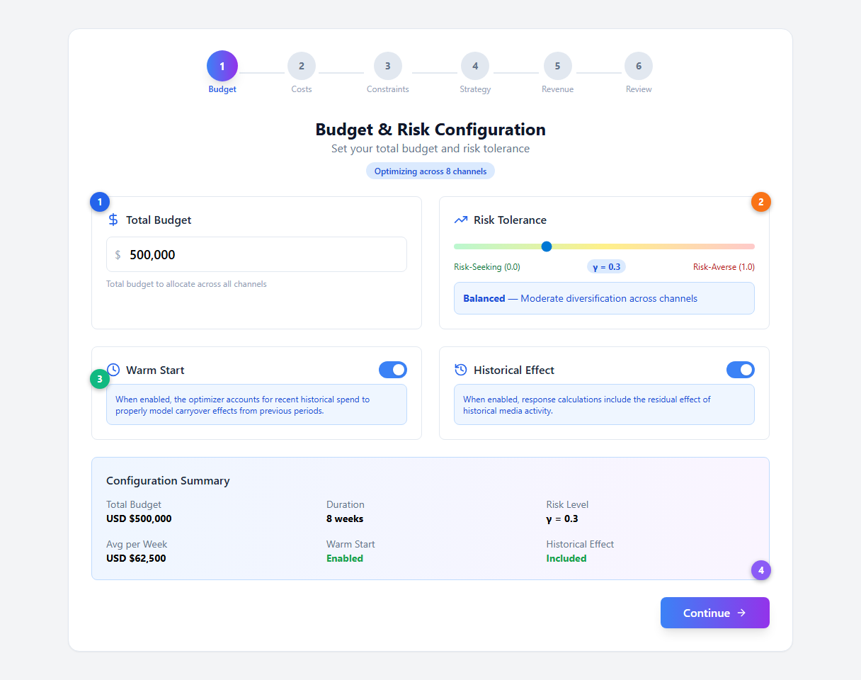
| # | Element | Description |
|---|---|---|
| 1 | Total Budget | The total amount to allocate across all channels for the planning period |
| 2 | Risk Tolerance (Gamma) | Slider from 0.0 to 1.0. Controls the tradeoff between maximizing expected return and diversifying to reduce uncertainty. See how gamma works |
| 3 | Warm Start & Historical Effect | Warm Start accounts for adstock carryover from previous periods. Historical Effect includes residual media effects |
| 4 | Summary panel | Live preview of all configuration settings |
Risk Tolerance in detail:
The gamma parameter controls how the optimizer balances return against uncertainty:
| Gamma Range | Behaviour | When to Use |
|---|---|---|
| 0.0 — 0.2 (Risk-Seeking) | Concentrates budget on highest-performing channels regardless of uncertainty | When you trust the model estimates and want maximum expected return |
| 0.3 — 0.7 (Balanced) | Moderate diversification. Balances expected return with stability | Default for most use cases. Good starting point |
| 0.8 — 1.0 (Risk-Averse) | Spreads budget to minimize variance. Prioritises reliable channels | When posterior uncertainty is high or you want conservative allocation |
The optimizer maximizes: E[response] — gamma x STD[response] across all posterior samples from your Bayesian model. This is a mean-variance objective function inspired by Modern Portfolio Theory.
Technical note: The UI gamma range (0 — 1) is scaled internally before optimization. Even small gamma values produce meaningful diversification because the penalty is applied to the standard deviation of the full posterior distribution.
Step 2: Configure Channel Costs
Define how each channel is costed.
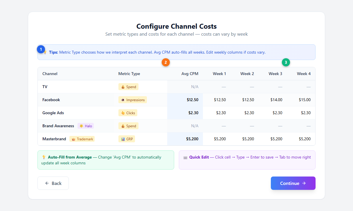
| # | Element | Description |
|---|---|---|
| 1 | Info tips | Guidance on metric types, average costs, and per-week editing |
| 2 | Metric Type | Dropdown per channel: 💰 Spend, 👁️ Impressions, 👆 Clicks, 📊 GRP, 📈 TRP. Halo (🌟) and Trademark (👑) channels are badged |
| 3 | Avg CPM / per-week columns | Blue-highlighted average column auto-fills all weeks. Edit individual weeks for seasonal cost variation |
Simba supports five metric types:
| Metric Type | Cost Field | Description |
|---|---|---|
| Spend | N/A | Direct spend-based (no conversion needed) |
| Impressions | CPM (cost per thousand) | Set per-period CPMs to account for seasonal variation |
| Clicks | CPC (cost per click) | For search and display channels |
| GRP | CPP (cost per point) | For traditional TV buys |
| TRP | CPP (cost per point) | For targeted TV buys |
Per-period cost columns let you account for seasonal CPM variation (e.g., higher costs during Q4). Editing the average cost auto-fills all period columns.
Step 3: Channel Constraints
Set minimum and maximum spend bounds for each channel as percentages of total budget.
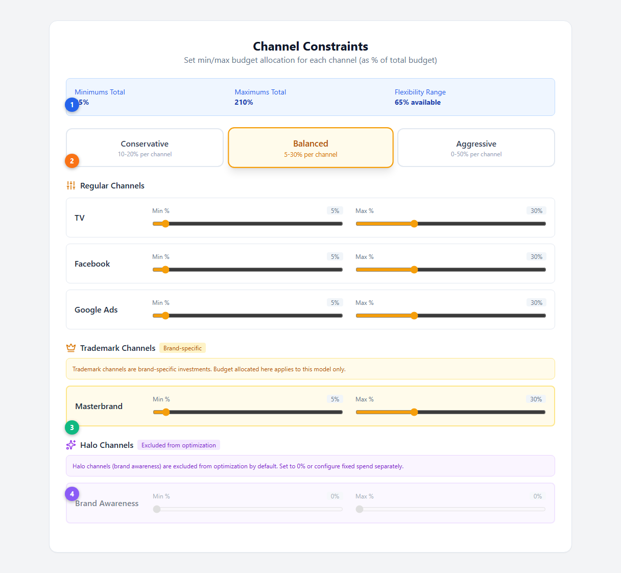
| # | Element | Description |
|---|---|---|
| 1 | Preset buttons | Quick-apply Conservative (10 — 20%), Balanced (5 — 30%), or Aggressive (0 — 50%) bounds |
| 2 | Channel sliders | Set minimum and maximum % of total budget per channel |
| 3 | Halo channels | Automatically excluded (0 — 0% bounds) since they represent brand awareness spillover, not directly optimisable spend. See Halo Effects |
| 4 | Validation summary | Real-time check that constraints are feasible: minimums total, maximums total, and flexibility range |
Constraint presets:
| Preset | Min | Max | Best For |
|---|---|---|---|
| Conservative | 10% | 20% | Stable allocation with limited channel swings |
| Balanced (default) | 5% | 30% | Good flexibility while preventing extreme concentration |
| Aggressive | 0% | 50% | Maximum optimizer freedom. Use when you trust the model |
Validation rules:
- If minimums exceed 100%, an error blocks you from continuing (the optimizer cannot satisfy all minimums within budget).
- If maximums are too restrictive, the optimizer may not have enough flexibility to improve on equal allocation.
- A warning appears if minimums exceed 85% of total budget (limited flexibility).
Step 4: Laydown Strategy (Multi-Period Only)
Choose how budget is distributed across the planning periods. This step is skipped when optimising a single period.
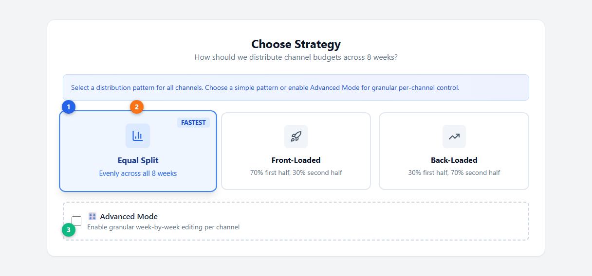
| # | Element | Description |
|---|---|---|
| 1 | Strategy cards | Choose how budget is distributed across planning periods |
| 2 | Selected strategy | Blue border, elevated shadow, and scale effect indicate selection |
| 3 | Advanced Mode | Enable per-channel, per-week weight editing in a detailed grid |
Available strategies:
| Strategy | Distribution | When to Use |
|---|---|---|
| Equal Split (Fastest) | Evenly across all periods | Default. Good for sustained activity |
| Front-Loaded | 70% first half, 30% second half | Product launches, seasonal ramp-ups |
| Back-Loaded | 30% first half, 70% second half | Building toward a peak event (e.g., Black Friday) |
Advanced Mode enables granular week-by-week editing per channel in a grid. Each channel’s weights must sum to 100%. Edit the “Total” cell to auto-rebalance.
Step 5: Configure Revenue Conversion
Set a multiplier to convert the model’s target variable into revenue.
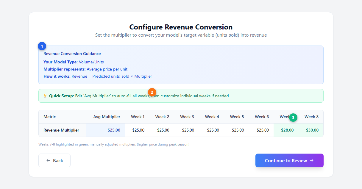
| # | Element | Description |
|---|---|---|
| 1 | Guidance card | Shows your model type (Volume/Units, Customers, Revenue) and what the multiplier represents |
| 2 | Quick Setup tip | Edit ‘Avg Multiplier’ to auto-fill all weeks |
| 3 | Multiplier table | Blue-highlighted average column. Green-highlighted cells show manually adjusted weeks (e.g., higher prices during peak season) |
| Model Type | Multiplier Represents | Example |
|---|---|---|
| Volume / Units | Average price per unit | $25.00 per unit |
| Customer / Acquisition | Customer lifetime value (LTV) | $500.00 LTV |
| Revenue / Sales | No conversion needed | 1.0 (already in revenue) |
Multipliers can vary by period to account for seasonal pricing or expected conversion rate changes. Editing the average auto-fills all period columns.
Step 6: Review & Run
Review all configuration settings and launch the optimisation.
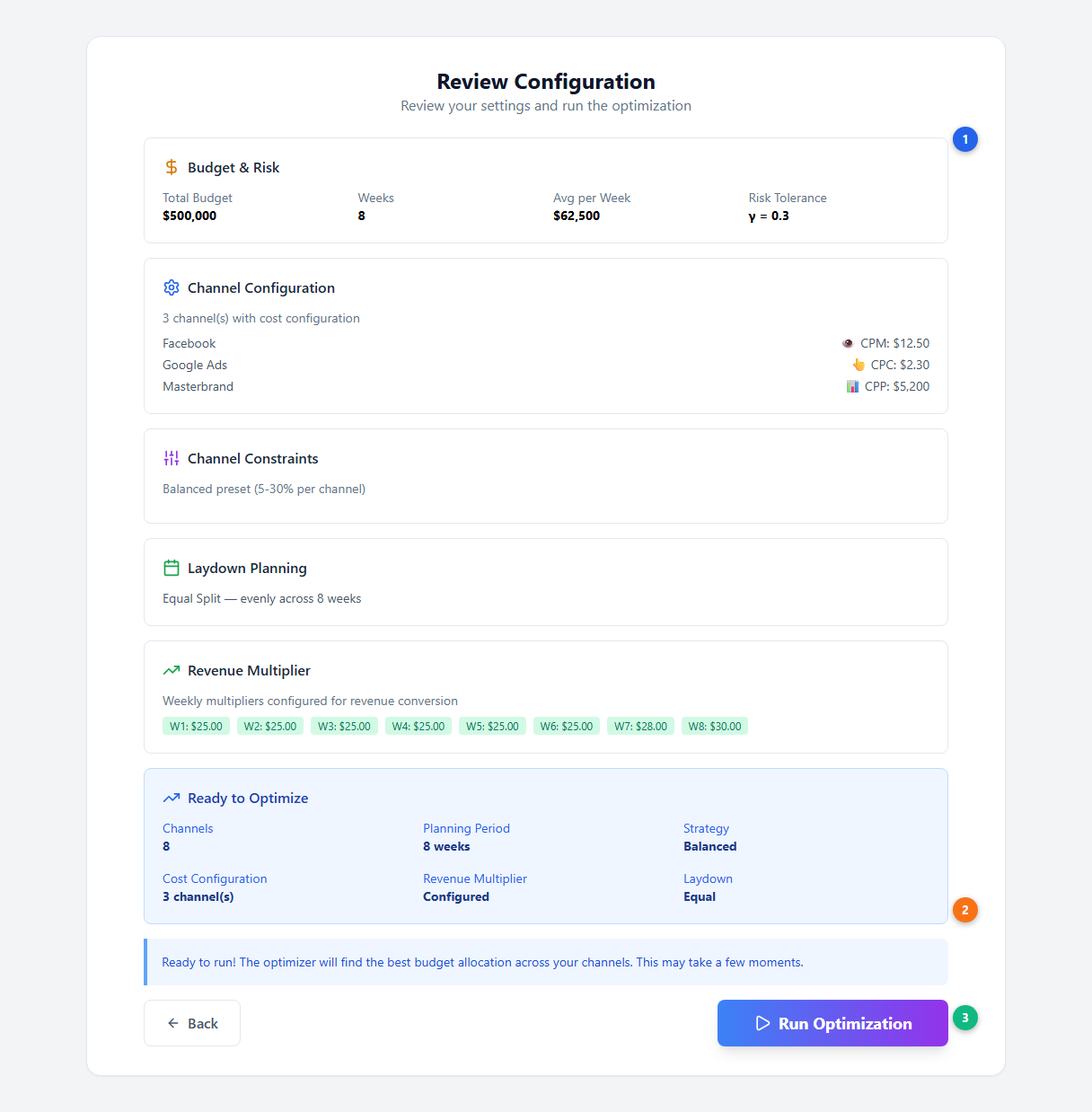
| # | Element | Description |
|---|---|---|
| 1 | Configuration summary | All settings from steps 1 — 5 displayed in collapsible cards |
| 2 | Ready panel | Summary of key parameters at a glance before running |
| 3 | Run Optimization | Launches the optimizer with a progress bar showing completion percentage |
After clicking Run Optimization, a progress bar shows real-time completion status with descriptive messages.
How the Optimizer Works
The optimizer uses scipy’s constrained optimization to solve for the budget allocation that maximizes the risk-adjusted objective across all posterior samples from the Bayesian model.
It accounts for:
- Diminishing returns: Each additional dollar spent on a channel produces less incremental revenue as the channel approaches saturation. The optimizer spreads budget across channels to capture the most efficient marginal returns.
- Carryover effects: Adstock decay curves mean that spend in one period continues generating response in subsequent periods. When Warm Start is enabled, the optimizer accounts for historical spend bleeding into the planning window.
- Uncertainty: The gamma parameter controls how much the optimizer penalises channels with wide posterior distributions (high uncertainty in their response estimates).
- Constraints: Per-channel percentage bounds, total budget constraint, and laydown weights are all enforced simultaneously.
For a deeper explanation of the mathematics behind this — marginal response curves, the efficient frontier, and the mean-variance framework — see Optimization (Core Concepts).
Interpreting Optimization Results
After the optimizer completes, the results page shows a comprehensive breakdown.
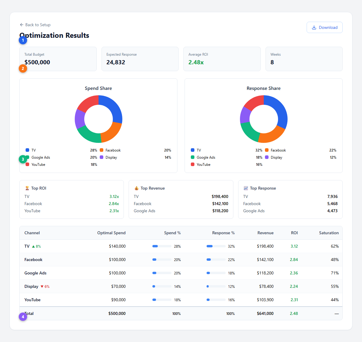
| # | Element | Description |
|---|---|---|
| 1 | KPI header cards | Total budget, expected response, average ROI, and planning weeks at a glance |
| 2 | Share comparison | Spend Share vs Response Share donuts. Channels earning more response than their spend share are high-efficiency |
| 3 | Top Insights | Top 3 channels by ROI, revenue, and response for a quick executive summary |
| 4 | Results table | Full per-channel breakdown with spend, shares, revenue, ROI, and saturation level. Expandable rows show weekly detail |
Results Table Columns
| Column | Description |
|---|---|
| Channel | Channel name (click to expand for weekly detail) |
| Optimal Spend | Recommended spend allocation |
| Spend % | Percentage of total budget with visual bar |
| Response % | Percentage of total expected response with visual bar |
| Revenue | Expected revenue (response multiplied by your multiplier) |
| ROI | Return on investment. Color-coded: green (>= 1.0), amber (>= 0.5), red (< 0.5) |
| Saturation | Saturation level at the recommended spend. Higher % means the channel is closer to its ceiling |
Reading the Donuts
Compare Spend Share with Response Share to identify efficiency:
- A channel with 15% spend share but 25% response share is under-saturated — it delivers disproportionate value and may benefit from more budget. This corresponds to operating in the steep region of the saturation curve.
- A channel with 25% spend share but 15% response share is over-saturated — budget could be shifted elsewhere for better returns. This corresponds to operating in the flat region of the saturation curve.
Weekly Flighting Chart
Below the table, a metric toggle (Response / Revenue) switches the weekly stacking chart view:
- Weekly Spend bars show how each channel’s budget is distributed across planning periods.
- Weekly Response bars show the expected response per period, including adstock carryover tail periods beyond the planning window (labeled Tail 1, Tail 2, etc.). This visualises how the effects of spend persist after the campaign ends.
Acting on Recommendations
Optimization results are recommendations, not automatic actions:
- Review with your media team. Check whether the suggested changes are operationally feasible (minimum buys, platform constraints, creative availability).
- Apply business constraints. If there are contractual commitments or strategic mandates, add these as constraints in Step 3 and re-run.
- Phase large changes. If the optimizer recommends a major shift, consider implementing in stages and monitoring actual performance.
- Close the loop. After implementing, feed new performance data back into Simba. Run Incremental Measurement to update attribution, and the cycle continues.
Portfolio Optimization
When optimising at the portfolio level, the optimizer accounts for cross-brand effects:
- Halo channels generate lift not just for their primary brand but for other brands in the portfolio. The optimizer gives them credit for total portfolio impact.
- Trademark channels (masterbrand, portfolio, corporate) are optimised against total revenue across all brands, not attributed to any single brand.
The optimizer solves for the allocation that maximises total portfolio revenue, including direct channel effects, halo spillover, and trademark-level impact.
See Halo and Trademark Channels and Portfolio Analysis for configuration details.
Common Issues
| Issue | Cause | Solution |
|---|---|---|
| Constraint validation error | Per-channel minimums exceed the total budget (sum of minimums > 100%) | Reduce minimum bounds so they sum to less than the total budget |
| Warning: minimums exceed 85% | Very little room for the optimizer to reallocate spend | Loosen minimum constraints to give the optimizer more flexibility |
| Optimizer returns current allocation | Channels are already near-optimal, or constraints are so tight the optimizer has no room to move | Widen the min/max bounds, or increase the total budget to create reallocation headroom |
| All channels at minimum bounds | High risk aversion (gamma) combined with wide uncertainty spreads across allocation equally | Reduce gamma to allow the optimizer to concentrate spend where returns are higher |
| Unexpected channel getting most budget | That channel has the steepest marginal return curve at current spend levels | Review the saturation curves for that channel — it may be far from saturation, making additional spend highly efficient |
Next Steps
Platform guides:
- Scenario Planning — Test budget scenarios before optimising
- Model Configuration — Adjust the underlying model parameters
- Incremental Measurement — The attribution results that drive optimization
- Portfolio Analysis — Cross-brand optimization
Core concepts:
- Optimization — The theory behind marginal response curves, the efficient frontier, and risk-adjusted allocation
- Saturation Curves — How diminishing returns shape the optimizer’s recommendations
- Adstock Effects — How carryover dynamics affect multi-period optimization
- Halo Effects — Cross-brand effects in portfolio optimization