Simba documentation

Quick Start Guide — Build Your First Marketing Mix Model

This guide walks you through the complete Simba workflow, from signing up to interpreting your first optimized budget recommendation. By the end, you will have a working Bayesian marketing mix model with actionable channel-level insights.

Quick start steps

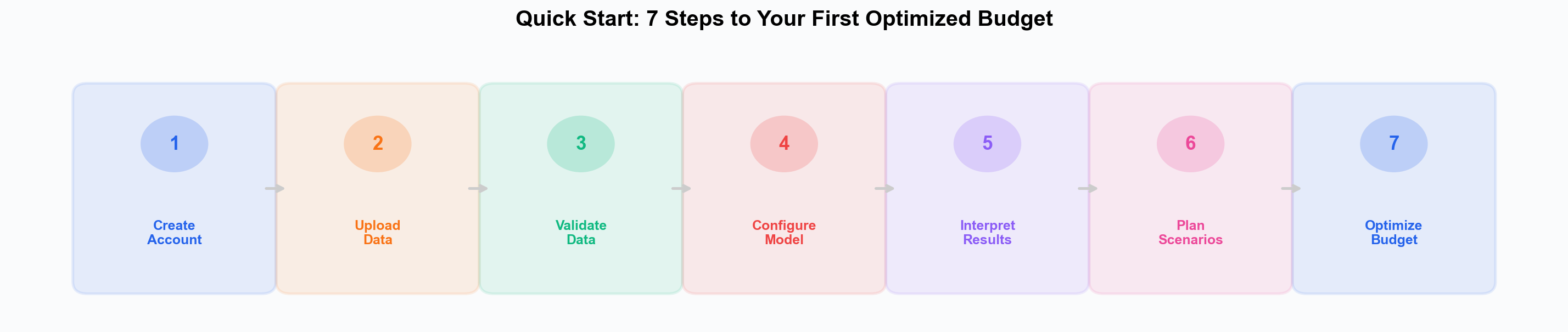
Time required: Most users complete their first model run within a few hours. The actual computation takes minutes; the majority of your time will be spent reviewing data and results.

Before you start: Make sure you have prepared your data as a CSV with date, media spend, and a target KPI column (weekly or daily granularity). Need a refresher on what Simba does? Read What is Simba? first.

Step 1: Create Your Account

Start free: register with your email, or sign up with Google or Microsoft. Prefer a walkthrough first? Book a demo.
Click the confirmation link in your inbox, then sign in.
You land in the Trial plan: a 28-day free trial with access to core features, and a sample model fitted on synthetic data already in your Default Project.
No credit card and no approval step are required to start.

For detailed information about plans, projects, and team setup, see Account Setup.

Step 2: Prepare and Upload Your Data

Prepare your data

Simba expects a time-series dataset in CSV format with:

A date column (weekly or daily granularity)
One or more media spend or activity columns (e.g., tv_spend, paid_search_spend, social_impressions)
A target KPI column (e.g., revenue, conversions, leads)
Optional: control variables (e.g., price, promotions, seasonality_flag, competitor_activity)

A clean dataset with 1 to 3 years of weekly data is ideal for most use cases. See Data Preparation for a full guide on formatting, granularity, and common pitfalls.

Upload your data

From the Model Warehouse, click New Model or navigate to the data upload screen.
Drag and drop your CSV file or click to browse.
Simba will parse your file and display a preview of the detected columns.
Map your columns: select which column is the date, which are media channels, which is the target KPI, and which are control variables.

Tip: Name your CSV columns clearly (e.g., paid_search_spend rather than channel_3). Simba uses column names in all charts and reports.

Step 3: Run the Data Validator

Before building a model, Simba’s Data Validator automatically reviews your dataset. This step is part of the Audit phase of the Simba workflow.

The auditor checks for:

Missing values — gaps in your time series that could bias results
Outliers — extreme values that may distort model estimation
Multicollinearity — channels whose spend patterns are too correlated, making it difficult to disentangle their effects
Stationarity and trends — structural changes in your data over time
Data quality issues — formatting errors, zero-variance columns, or insufficient data length

You will receive a clear audit report with a health score and specific recommendations. Address any critical issues before proceeding. Many issues can be resolved directly in Simba’s data preparation tools.

Step 4: Configure Your Model

This is the Measure phase. Simba needs to know how to model the relationship between your marketing channels and your KPI. There are three key configuration areas:

Priors

Priors express what you believe about each channel’s effect before seeing the data. For example, you might believe that TV has a positive but uncertain effect on revenue. Simba lets you set prior distributions through the UI — no code needed.

Smart Defaults: Simba auto-generates sensible priors from your historical data. For your first model, we recommend starting with the smart defaults and refining later. This gets you to results quickly while maintaining statistical validity.

Adstock (Carryover Effects)

Marketing does not always have an immediate effect. A TV ad aired on Monday may drive searches and conversions throughout the week. Adstock parameters control how each channel’s effect decays over time. Simba provides geometric and delayed adstock options, configurable per channel via the UI.

Smart defaults will suggest appropriate adstock settings based on channel type and your data patterns.

Saturation (Diminishing Returns)

At some point, spending more on a channel yields diminishing returns. Saturation curves model this effect. Simba uses the tanh saturation function, configurable per channel.

Smart defaults estimate saturation parameters from the observed spend ranges in your data.

Running the model

Once you are satisfied with your configuration (or have accepted the smart defaults):

Review the model summary panel, which shows your selected priors, adstock, and saturation settings.
Click Run Model.
Simba will run the Bayesian inference using PyMC-Marketing. This typically takes a few minutes depending on dataset size and model complexity.
You will see a progress indicator and be notified when the run completes.

Step 5: Interpret Your Results

When the model finishes, you will land on the Active Model page. Here is what to look at first:

Channel Contributions

The channel contribution chart shows how much each marketing channel (and baseline/control factors) contributed to your KPI over the modeled period. Unlike deterministic tools, Simba shows you 94% credible intervals (HDI) — the range of plausible contribution values — not just a single number.

Return on Ad Spend (ROAS)

Simba calculates the posterior ROAS for each channel, telling you how much KPI return you get for each unit of spend. Channels with wide 94% credible intervals (HDI) have more uncertainty — this is honest reporting, not a flaw.

Adstock and Saturation Curves

Visualize how each channel’s effect decays over time (adstock) and how it responds to increased spend (saturation). These curves are essential for understanding channel dynamics.

Model Diagnostics

Check the model fit, convergence diagnostics, and posterior predictive checks. These tell you whether the model adequately captures your data patterns. Simba highlights any issues and provides plain-language explanations.

Step 6: Plan Scenarios

With a fitted model, move to the Predict phase. Scenario Planning lets you simulate changes to your budget and see the predicted impact:

Navigate to Scenario Planning from the results screen.
Adjust channel budgets using the sliders or input fields. For example, increase paid social by 20% and decrease TV by 10%.
Click Simulate to see the predicted KPI outcome with uncertainty intervals.
Compare multiple scenarios side by side.

This is where Simba moves beyond measurement into decision support. You can test hypotheses before committing real budget.

Step 7: Optimize Your Budget

The final step is the Optimize phase. Budget Optimizer automatically finds the best allocation:

Navigate to Budget Optimizer from the scenario planning screen or main navigation.
Set your total budget constraint (the total amount you have to allocate).
Optionally set per-channel minimum and maximum spend constraints (e.g., “TV must be at least 10% of total”).
Choose your optimization objective (maximize revenue, conversions, etc.).
Click Optimize.
Simba returns the recommended allocation with the expected KPI lift compared to your current spend.

The optimization is grounded in the full posterior distribution of your Bayesian model, meaning it accounts for uncertainty in channel effects rather than optimizing against a single point estimate.

What to Do Next

Congratulations — you have built, interpreted, and optimized your first Bayesian marketing mix model. Here are recommended next steps:

Refine your priors. Now that you have seen the results, consider whether the smart defaults align with your domain knowledge. Adjust priors and re-run to see how results change. See Setting Priors.
Add control variables. If you did not include price, promotions, or seasonality controls, adding them can improve model accuracy. See Control Variables.
Explore model diagnostics. Dive deeper into convergence, posterior predictive checks, and sensitivity analysis. See Model Diagnostics.
Set up regular updates. As new data comes in, re-run your model to keep insights current. Simba preserves your configuration for easy re-runs.
Invite your team. Share results and collaborate on scenarios. See Account Setup for team management.
Prepare your data. If you need to clean or format your data, see the Data Preparation guide.
Try VAR modeling. For multi-variable time series analysis that captures inter-channel dynamics, explore VAR Models.

Troubleshooting

Issue	Solution
Data upload fails	Check that your file is a valid CSV with a header row and is under 10 MB. Excel (.xlsx) is not supported. See Data Requirements.
Data Validator flags critical issues	Address the flagged issues in your data before running the model. The audit report includes specific guidance for each category.
Model takes too long	Large datasets or complex configurations increase run time. Try reducing the number of channels, using weekly instead of daily data, or disabling seasonality/trend.
Model status “Failed”	Check the error message. Common causes: too few observations for the number of parameters, conflicting priors (e.g., very tight priors that disagree with data), or data quality issues the validator didn’t catch. Fix the underlying issue and re-run.
Model status “Time Exceeded”	The model exceeded maximum computation time. Simplify by reducing channels, using weekly data, or turning off optional features (seasonality, trend, weekly seasonality).
R-hat warnings (> 1.1)	The model did not fully converge. Try increasing the number of MCMC samples, simplifying the model (fewer channels, simpler priors), or checking for multicollinearity in your data. See Measurement diagnostics.
Optimizer returns current allocation unchanged	Channels may already be near-optimal, or per-channel constraints are too tight. Try widening the min/max bounds in the constraint step.
Poor model fit	Review diagnostics and consider adding control variables, adjusting priors, or checking data quality. A poor fit often means the model is missing an important driver (seasonality, promotions, competitor activity). See Model Diagnostics.
Results seem unreasonable	Check your priors and data. Common causes: overly vague priors allowing unrealistic coefficients, missing control variables that inflate channel credit, or data errors. See Setting Priors.

For additional help, open a GitHub issue or email info@pymc-labs.com.

Your First Model — Hands-on tutorial with sample data
What is Simba? — Understand the platform and methodology
Account Setup — Plans, projects, and team management
Platform Overview — Navigate the full interface
Data Requirements — Detailed data preparation guide
Bayesian Modeling in Marketing — The theory behind the engine

This site is open source. Improve this page.