Simba documentation
Long-Term Effects — Interpreting Lasting Brand Impact
Standard Marketing Mix Models measure short-term media impact: the incremental revenue generated within a few weeks of adstock decay. But some marketing activities — brand campaigns, sponsorships, sustained awareness efforts — produce effects that persist for months or longer. The Long-Term Effects module captures this extended impact using Vector AutoRegression (VAR) to trace how marketing spend flows through brand-building variables (awareness, consideration, equity) to ultimately drive revenue, complementing the saturation and carryover modeling of your standard MMM.
Prerequisites: Long-run effects require a trained VAR model with at least 2 endogenous variables and 1 exogenous variable, and a configured long-run effects analysis. For setup instructions, see VAR Models. For linking a VAR to your MMM model, see VAR Models — Linking.
The VAR Analysis Trio
When you build a VAR model in Simba, the results page includes seven tabs. The last three — Impulse Response, Variance Decomposition, and Long-Run Effects — form a connected analysis workflow for understanding long-term marketing impact.
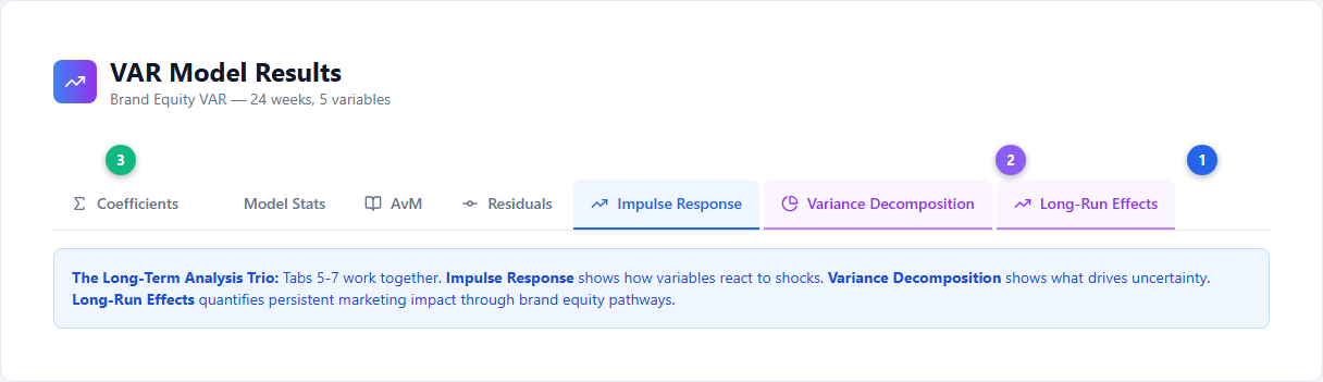
| # | Element | Description |
|---|---|---|
| 1 | Long-Run Effects tab | Quantifies persistent marketing impact through brand equity pathways — the primary output for budget decisions |
| 2 | Variance Decomposition tab | Shows what drives uncertainty in each variable — which channels matter most at different time horizons |
| 3 | Standard VAR tabs | Coefficients, Model Stats, AvM, and Residuals — standard model diagnostics |
These three tabs work together: IRF shows how variables respond to shocks, FEVD shows what drives uncertainty, and Long-Run Effects quantifies the persistent cumulative impact on your base metric.
Interpreting Impulse Response Functions
Impulse Response Functions (IRFs) show how each variable responds over time when another variable receives a sudden one-unit “shock”. This is the foundation for understanding how marketing spend ripples through your brand metrics. Unlike standard MMM priors which capture short-term response shapes, IRFs reveal the full dynamic system of cross-variable effects.
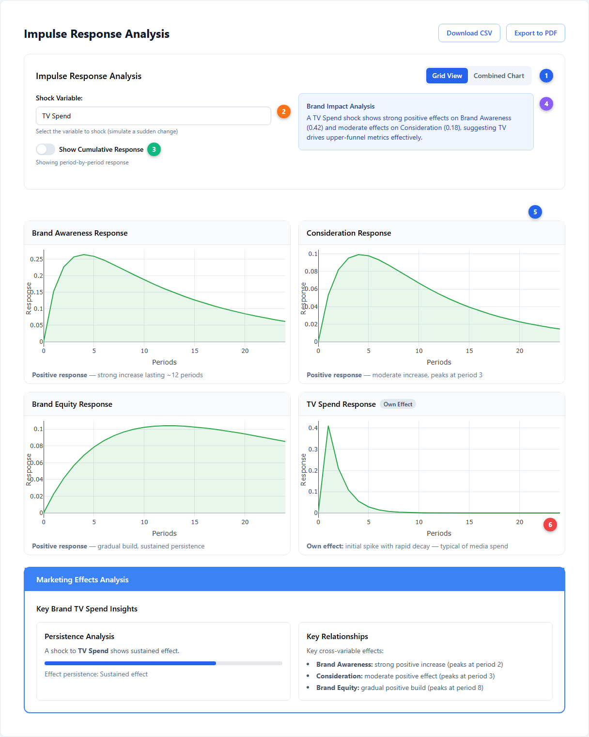
| # | Element | Description |
|---|---|---|
| 1 | Grid / Combined toggle | Grid View shows each response in its own chart; Combined Chart overlays all responses for comparison |
| 2 | Shock Variable selector | Choose which variable to “shock” — typically a media spend channel — to see how all other variables respond |
| 3 | Cumulative toggle | Off = period-by-period response; On = total accumulated effect over time. Cumulative mode shows the building long-run impact |
| 4 | Brand Impact Analysis | Auto-generated insight summarizing the key cross-variable effects of the selected shock |
| 5 | Response chart grid | 2-column responsive grid of Plotly charts (one chart per variable). Green (#28a745) = positive response, Red (#dc3545) = negative response. Fill shows direction clearly |
| 6 | Own Effect badge | Marks the chart showing how the shocked variable responds to itself — typically a spike with rapid decay for media spend |
Tip: Use the Download CSV and Export to PDF buttons in the header to save IRF results for reports and presentations.
Reading IRF Charts
- Green (positive) responses mean the variable increases after the shock — e.g., TV spend increases brand awareness
- Red (negative) responses mean the variable decreases — rare but possible (e.g., heavy discounting could hurt brand equity)
- Persistence: how long the effect lasts before returning to zero. Short-lived (<20% remaining after 5 periods) vs. long-lasting (>80%)
- Own effect: the shocked variable’s response to itself. Media spend typically shows a sharp spike and rapid decay. Brand metrics may show self-reinforcing persistence
- Cross effects: how other variables respond. The magnitude, direction, and timing reveal the causal chain from spend to revenue
Cumulative Mode
Toggle cumulative mode on to see the total accumulated effect over time. This is the most relevant view for budget decisions — it shows how much total impact builds up rather than the period-by-period response. A channel whose cumulative curve keeps rising has strong persistent effects worth investing in.
Marketing Effects Analysis
Below the chart grid, the Marketing Effects Analysis panel provides automated interpretation:
- Persistence Analysis: A visual bar showing what percentage of the initial shock effect remains after a set number of periods. Short-lived effects (<20%) indicate performance-oriented channels; long-lasting effects (>80%) indicate brand-building channels
- Key Relationships: Up to 3 of the most significant cross-variable effects, ranked by magnitude. Each describes the direction (positive/negative), strength, and timing of the response
- Marketing Insight: A summary card synthesizing the overall pattern — whether the shocked variable primarily drives direct results or builds long-term brand value
Learning resource: Click the Show Explanation button at the bottom of the IRF section for an in-app educational guide explaining how IRFs work, with badge indicators showing positive (↑ green) and negative (↓ red) response interpretations.
Interpreting Variance Decomposition
Forecast Error Variance Decomposition (FEVD) answers: “what proportion of the uncertainty in each variable is explained by shocks to each other variable?” This reveals which channels and metrics are the dominant drivers of your outcome variable.
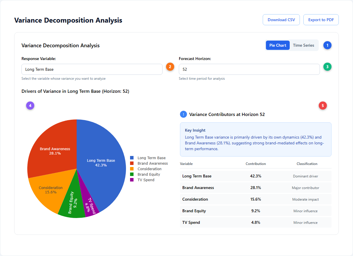
| # | Element | Description |
|---|---|---|
| 1 | Pie / Time Series toggle | Pie Chart = snapshot at one horizon; Time Series = stacked bar showing how contributions evolve over time |
| 2 | Response Variable selector | Choose which variable’s variance to decompose (typically your base/revenue variable) |
| 3 | Forecast Horizon selector | How far into the future to measure variance contributions. Longer horizons reveal more about persistent effects |
| 4 | Pie chart | Color-coded breakdown using a 20-color palette. Labels show both variable name and percentage contribution |
| 5 | Insights panel | Auto-classified contributions with emoji indicators: dominant (✓), moderate (~), minor (-). Shows top 5 contributors with narrative insight |
Tip: Use the Download CSV and Export to PDF buttons to save FEVD results. Click Show Explanation at the bottom for an in-app educational guide with tips (highlighted in yellow) on interpreting variance decomposition.
Reading FEVD Results
| Classification | Threshold | What it means |
|---|---|---|
| Dominant driver | ≥60% | This variable explains most of the uncertainty — focus optimization here |
| Major contributor | ≥30% | Significant influence — meaningful lever for improvement |
| Moderate impact | ≥10% | Worth monitoring but not the primary driver |
| Minor influence | <10% | Limited contribution to variance at this horizon |
Pie vs Time Series: Use Pie Chart for a quick snapshot at a specific horizon. Switch to Time Series (stacked bar) to see how contributions evolve over time — variables whose share grows at longer horizons have increasing long-run importance.
Note: FEVD is unavailable when Fast Mode is enabled during VAR training. Fast Mode uses a diagonal covariance matrix which skips the cross-variable covariance estimation needed for FEVD. To enable FEVD, rebuild the model with Fast Mode disabled. For Fast Mode configuration, see VAR Models.
Long-Run Effects Results
When the VAR model finishes training with long-run effects configured, the Long-Run Effects tab shows up to five sub-tabs of results. Each sub-tab includes Download CSV and Export to PDF buttons for reporting.
Configuration Summary
At the top of every sub-tab, a blue gradient card confirms your analysis settings:
| Field | What it shows |
|---|---|
| Base Variable | The target metric (e.g., long_term_base, revenue) |
| Equity Variables | Brand metrics that mediate effects (e.g., brand_awareness, consideration) |
| Horizon | Number of periods for cumulative analysis (default: 156 = ~3 years weekly) |
| Confidence | Width of Bayesian credible intervals (90%, 95%, or 99%) |
| Transformations | Whether media variable transformations were applied. If shown, a details panel lists per-channel transform types with ⚠ warnings for potentially problematic transformations (e.g., log with zeros) |
Exogenous scaling note: If exogenous scaling was enabled during VAR training, elasticities are interpreted as “per 1 standard deviation increase” rather than “per 1% increase”. A warning banner appears when this is the case.
Elasticities Tab (Default)
The primary results view showing each channel’s total persistent effect on your base variable.
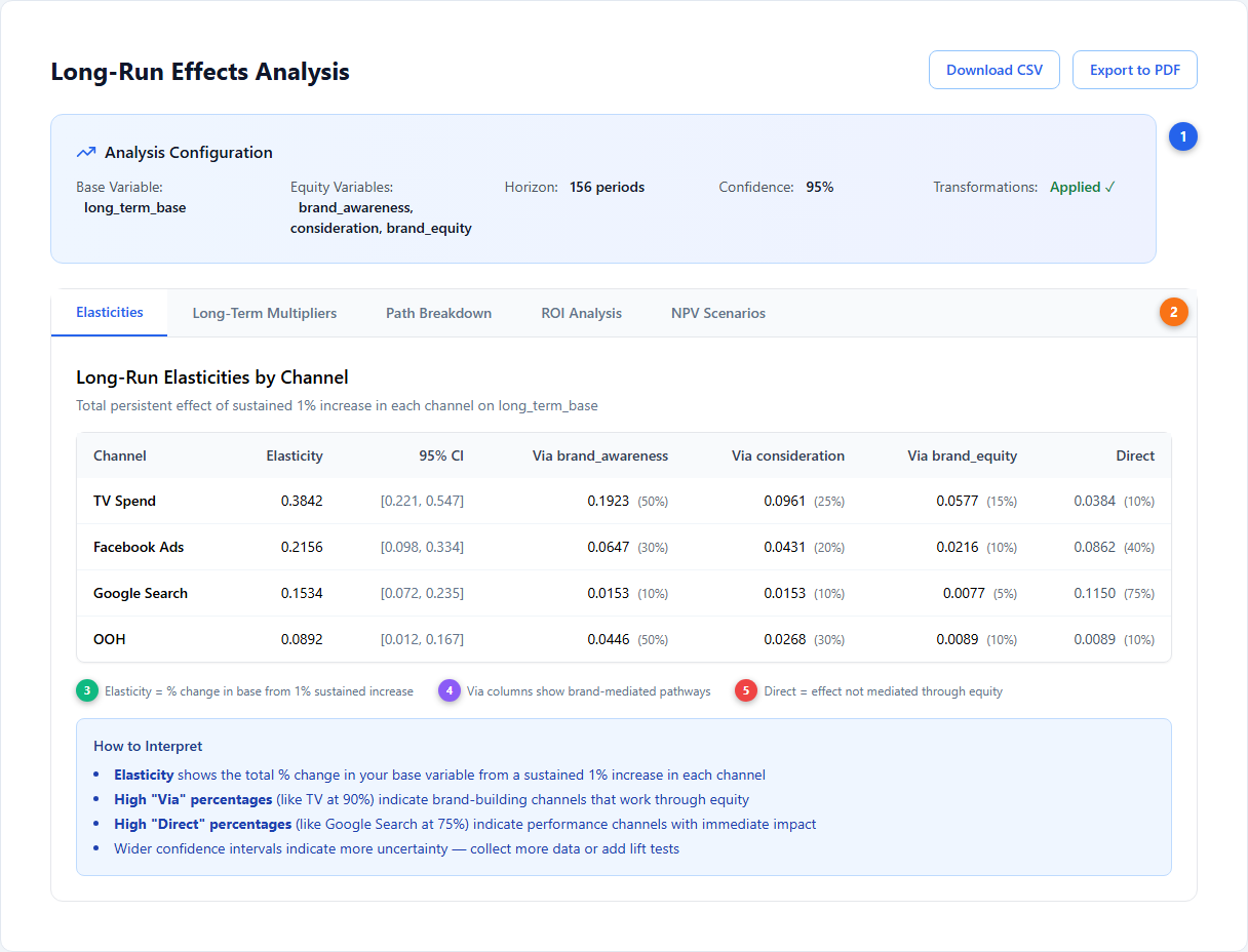
| # | Element | Description |
|---|---|---|
| 1 | Analysis Configuration summary | Blue gradient card confirming: base variable, equity variables, horizon, confidence level, and whether transformations were applied |
| 2 | Results sub-tabs | Five tabs: Elasticities (always), Long-Term Multipliers (always), Path Breakdown (always), ROI Analysis (conditional), NPV Scenarios (conditional) |
| 3 | Elasticity value | Total % change in your base variable from a sustained 1% increase in each channel. Higher = stronger long-run effect |
| 4 | Via columns | Show how much of the total effect flows through each equity pathway (brand_awareness, consideration, brand_equity). Percentages reveal brand-mediated vs performance impact |
| 5 | Direct column | Effect that bypasses brand metrics entirely — captures immediate/performance-oriented response |
How to interpret elasticities:
- Brand builders (like TV with 90% via equity): Most impact flows through brand metrics. These channels build long-term value that standard adstock decay misses. Consider increasing budget allocation beyond what short-term ROAS suggests
- Performance channels (like Google Search with 75% direct): Most impact is immediate and well-captured by the standard MMM. Long-run effects are smaller but still present
- Wider credible intervals: Indicate more uncertainty in the estimate. Collect more data or integrate lift tests to narrow them
- Elasticity magnitude: 0.38 means a sustained 1% increase in that channel drives a cumulative 0.38% increase in your base variable over the full horizon
- Comparing channels: Sort by elasticity to rank channels by total long-run impact. A channel with a lower short-term ROAS but higher long-run elasticity may be undervalued
Long-Term Multipliers Tab
Shows the cumulative persistent effect of each equity variable on your base metric.
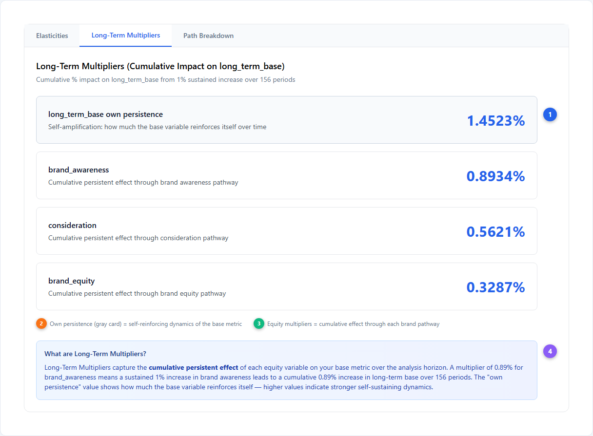
| # | Element | Description |
|---|---|---|
| 1 | Multiplier cards | One card per equity variable showing its cumulative persistent effect on the base variable |
| 2 | Own persistence (gray card) | Self-amplification: how much the base variable reinforces itself over time. Higher values indicate stronger self-sustaining dynamics |
| 3 | Equity multiplier values | A value of 0.89% means a sustained 1% increase in that equity variable leads to a cumulative 0.89% increase in the base over the analysis horizon |
| 4 | What are Long-Term Multipliers? | Explanation of long-term multipliers and how to interpret the cumulative persistence values |
How to interpret Long-Term Multipliers:
- Own persistence > 1: The base variable amplifies its own shocks — positive momentum effects
- High equity multipliers: These brand metrics are strong mediators of long-term value. Invest in channels that drive these metrics (revealed by the Path Breakdown tab)
- Low equity multipliers: These metrics have limited persistent effect on revenue, even if they respond strongly to marketing in the IRF view
- Comparing multipliers: The relative size tells you which brand dimensions matter most for your business. If brand_awareness has a 1.45% multiplier but consideration only 0.56%, awareness-building campaigns create more lasting value
Path Breakdown Tab
Shows how each channel creates long-term value — through which equity pathways.
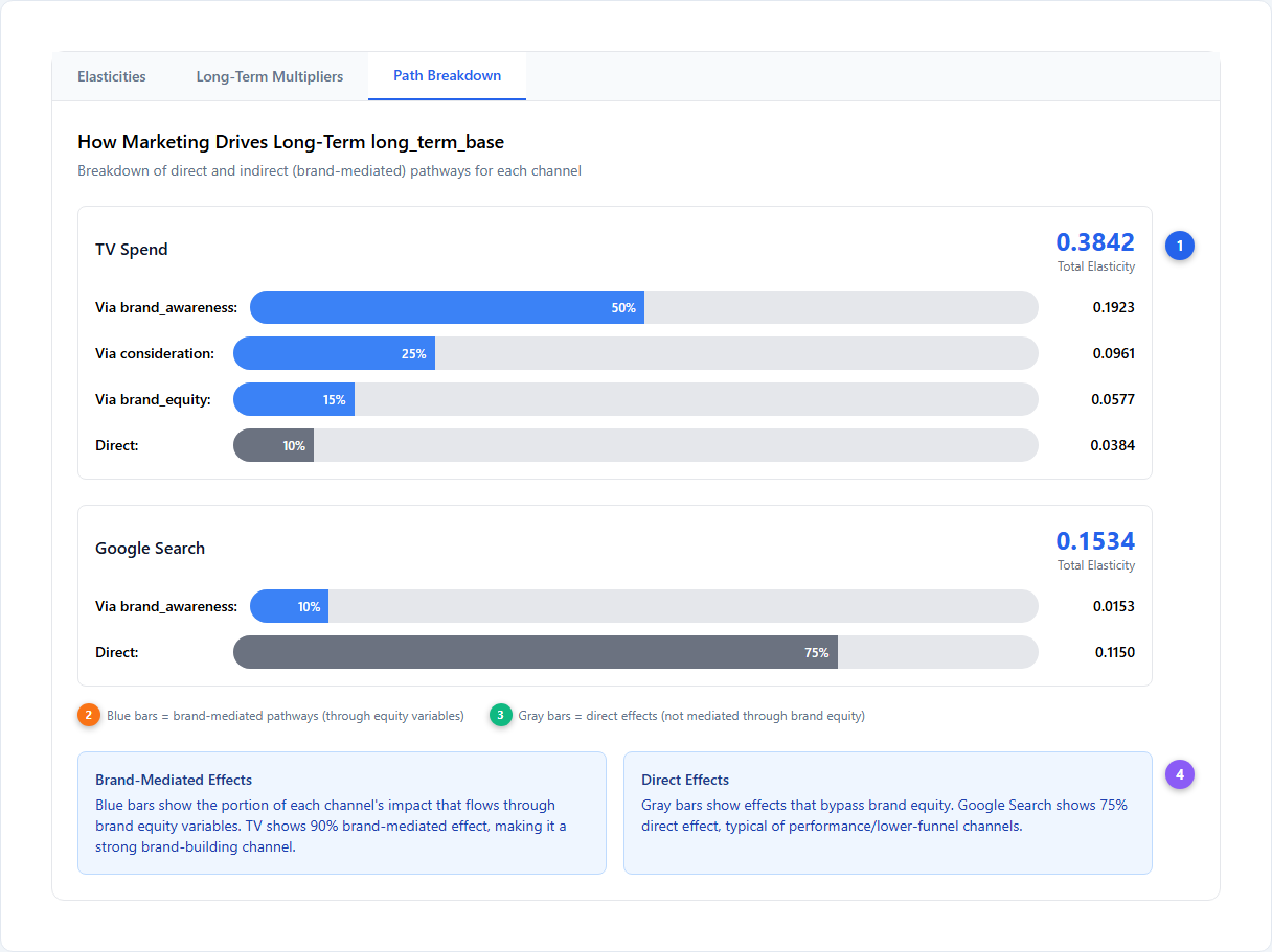
| # | Element | Description |
|---|---|---|
| 1 | Channel cards | One card per media channel showing total elasticity and the breakdown across pathways |
| 2 | Direct effect bar (gray) | The portion of the channel’s effect that bypasses brand metrics. Performance channels show dominant gray bars |
| 3 | Performance channel pattern | Google Search shows 75% direct effect — typical of lower-funnel channels where most value is immediate |
| 4 | Interpretation boxes | Two info boxes explaining brand-mediated effects and direct effects |
How to interpret Path Breakdown:
- Blue bars (Via equity) show brand-mediated pathways. TV’s 50% via brand_awareness means half its long-run impact flows through awareness
- Gray bars (Direct) show unmediated impact. High direct % = performance channel
- Multiple blue bars indicate a channel influences revenue through several brand metrics simultaneously — these are your most versatile brand-building channels
- Compare channels side-by-side to understand which drives awareness vs consideration vs equity
- Channel mix implications: If your brand is weak on consideration but strong on awareness, prioritize channels with higher Via consideration percentages
ROI Analysis Tab (Conditional)
Appears when annual spend and revenue data are provided during VAR configuration. Translates elasticities into long-run return on investment.
| Column | Description |
|---|---|
| Channel | Media channel name |
| Elasticity | Long-run elasticity (% per %) |
| PV Factor | Present value discount factor for multi-year horizon |
| Annual Spend | Your provided annual spend per channel |
| Long-Run ROI (NPV) | Net present value return on investment |
ROI color coding:
| Color | Threshold | Interpretation |
|---|---|---|
| Emerald (green) | ROI > 2x | Strong long-run return — channel pays for itself multiple times over |
| Blue | ROI > 1x | Positive long-run return — channel generates more value than it costs |
| Amber | ROI ≤ 1x | Weak or negative long-run return — consider reallocating budget |
How to interpret Long-Run ROI:
- Unlike short-term ROAS, Long-Run ROI accounts for the full cumulative impact through brand equity pathways, discounted to present value
- A channel with poor short-term ROAS but strong Long-Run ROI (>2x) is a brand builder whose value materializes over months — don’t cut it based on short-term metrics alone
- The PV Factor applies time-value-of-money discounting, so distant future effects are appropriately weighted lower than near-term effects
NPV Scenarios Tab (Conditional)
Appears when NPV scenario configuration is provided. Shows the present value of sustained marketing changes.
| Column | Description |
|---|---|
| Channel | Media channel name |
| Sustained Change | The percentage change you’re modeling (e.g., +10%) |
| Elasticity | Long-run elasticity applied to the change |
| NPV of Base Uplift | Total present value of the resulting base variable increase |
| Annual Value | Annualized impact for budgeting purposes |
How to interpret NPV Scenarios:
- NPV of Base Uplift answers: “If I sustain a 10% increase in TV spend for 3 years, what is the total present value of the resulting revenue increase?”
- Use this to build a business case for brand investment — translate percentage elasticities into monetary terms stakeholders understand
- Compare NPV across channels to identify where sustained investment creates the most value
- The Annual Value column helps translate lump-sum NPV into annual budget planning terms
Implications for Budget Decisions
Long-term effects fundamentally change how you think about budget optimization:
- Brand-building channels (high Via % in Path Breakdown) may warrant higher spend than short-term ROAS alone suggests, because their full return materializes over months through brand equity. Use the elasticities to quantify the gap between short-term and total return
- Performance channels (high Direct %) deliver most of their value immediately and are well-captured by standard MMM optimization with saturation curves
- Cutting brand spend saves money immediately but erodes the equity variables that support future revenue. The long-run elasticity quantifies exactly how much future revenue is at risk per % of spend reduction
- NPV analysis helps justify brand investment to stakeholders by translating long-run effects into financial terms with appropriate discounting
- Channel mix decisions: Compare Path Breakdown across channels to understand which drives awareness vs consideration vs equity, then align channel mix with your brand’s weakest equity dimension
- When linking VAR to MMM: The linked long-run effects automatically enhance your MMM’s measurement results, showing total (short + long) channel contributions rather than short-term only. For linking instructions, see VAR Models
Next Steps
Platform guides:
- VAR Models — Building, configuring, and linking VAR models in Simba
- Budget Optimization — How long-term effects influence allocation decisions
- Model Creation Wizard — Step-by-step model setup including VAR configuration
- Measurement — Channel attribution and results interpretation
Core concepts:
- VAR Modeling — Statistical foundation: Minnesota priors, IRF, FEVD, long-run multipliers
- Bayesian Modeling — The Bayesian approach and credible intervals
- Adstock Effects — Short-term carryover and decay (complementary to long-term effects)
- Saturation Curves — Diminishing returns in media response
- Priors & Distributions — Configuring Bayesian priors
- Incrementality — Causal attribution and lift test integration
Further Reading
- Cain, P. (2022). Modelling short- and long-term marketing effects in the consumer purchase journey. International Journal of Research in Marketing, 39(1), 96–116. — The foundational paper behind this approach: distinguishes short-term incremental sales response from long-term brand-building effects through the consumer purchase journey.