Simba documentation
Model Creation Wizard — Step-by-Step Model Setup
The Model Warehouse configuration tab guides you through a five-step wizard to create and configure a new marketing mix model. Each step builds on the previous, from data upload through to model fitting.
The Five-Step Wizard
The wizard follows this sequence:
- Source Configuration — Upload your CSV data and optionally validate it
- Model Setup — Choose between MMM and VAR model types
- Variable Selection — Categorize columns by role (media, cost, control, KPI, etc.)
- Prior Builder — Configure Bayesian priors for each variable
- Model Details — Set advanced options, lift tests, and start fitting
For MMM models, all five steps are used. For VAR models, the wizard flow differs — the model is configured and built from Step 2 with additional VAR-specific settings.
Step 1: Source Configuration
Upload your dataset and optionally run the Data Validator to check data quality before proceeding.
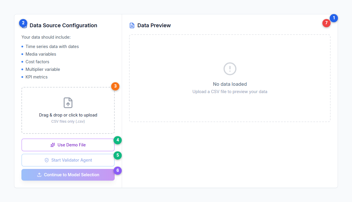
| # | Element | Description |
|---|---|---|
| 1 | Page header | Top-level section indicator for the wizard step |
| 2 | Data Source Configuration panel | Left column showing required data types: time series dates, media variables, cost factors, multiplier variable, and KPI metrics |
| 3 | CSV upload area | Drag & drop or click to upload. CSV files only (.csv), 10 MB maximum. Excel (.xlsx) is not supported |
| 4 | Use Demo File | Loads a sample 2-year marketing dataset for testing the platform without your own data |
| 5 | Start Validator Agent | Runs the Data Validator on your uploaded data using AI (disabled until a file is uploaded) |
| 6 | Continue to Model Selection | Proceeds to Step 2 (disabled until a file is uploaded) |
| 7 | Data Preview panel | Right column showing a preview table of your uploaded data with file name, size, column count, and sample rows |
Data Transformations
After uploading, an optional collapsible section lets you apply transformations to columns before modeling:
- Moving Average (window size 2–30, default 3)
- Adstock (Geometric Decay) (decay rate 0.01–0.99, default 0.7)
- Adstock (Delayed Peak) (alpha/bell width 0.01–0.99, default 0.7)
- Logarithmic
- Percentage Change
- Cumulative Sum
- Z-Score Normalization
These are optional data preparation transforms, not the model’s internal adstock or saturation functions.
Step 2: Model Setup
Choose your model type and configure high-level settings.
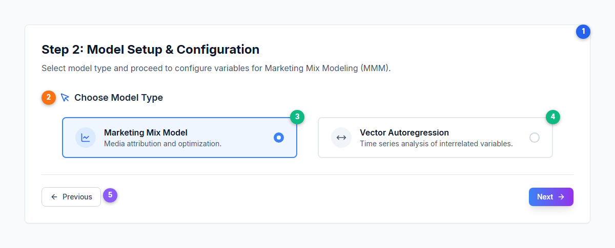
| # | Element | Description |
|---|---|---|
| 1 | Step header | “Step 2: Model Setup & Configuration” |
| 2 | Choose Model Type | Section for selecting between the two available model types |
| 3 | Marketing Mix Model (selected) | Standard MMM for channel attribution and optimization. Active state shown with blue border and background |
| 4 | Vector Autoregression | VAR model for analyzing inter-channel dynamics and time series relationships |
| 5 | Navigation buttons | Previous returns to Step 1, Next proceeds to Step 3 (Variable Selection) |
VAR Models
When VAR is selected, the wizard flow changes — additional configuration panels appear directly in Step 2 (lags, forecast horizon, endogenous/exogenous variables, media transformations, prior distributions) and the model is built from this step without proceeding through Steps 3–5.
For full details on setting up a VAR model, including the importance of correctly matching spend and media exposure variables, see VAR Models. For the underlying methodology, see VAR Modeling.
Step 3: Variable Selection
Categorize each column in your dataset by its role in the model using a three-panel layout. Correctly assigning variables is critical — media channels need matching cost variables for ROI calculations, and control variables should capture non-media factors that influence your KPI. For guidance on preparing your data before this step, see Data Requirements.
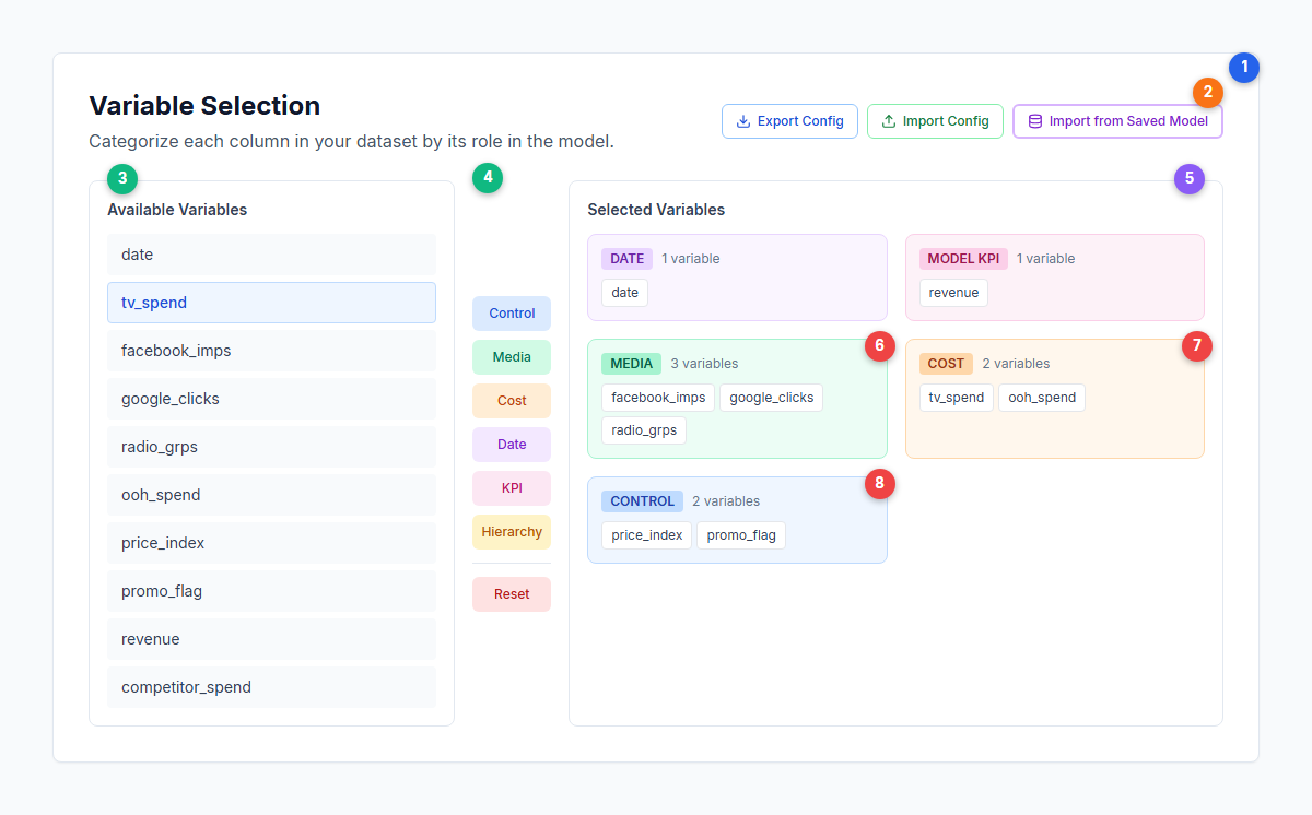
| # | Element | Description |
|---|---|---|
| 1 | Section header | “Variable Selection” with description |
| 2 | Config buttons | Export Config, Import Config, and Import from Saved Model — save/load variable assignments |
| 3 | Available Variables (left panel) | All columns from your uploaded CSV. Click to select, then assign using the category buttons |
| 4 | Category buttons (middle panel) | Assign selected variables to: Control, Media, Cost, Date, Multiplier, Model KPI, or Hierarchy. Reset clears all |
| 5 | Selected Variables (right panel) | Shows assigned variables grouped by category with color-coded cards |
| 6 | Media category | Green card showing assigned media channel variables |
| 7 | Cost category | Orange card showing assigned cost/spend variables |
| 8 | Control category | Blue card showing assigned control variables (non-media factors) |
Smart Variable Categorization
Simba uses AI-powered semantic matching to automatically suggest variable categorizations based on column names. The system recognizes 15 channel types (TV, Social, Search, Video, OOH, etc.) and 8 metric types (spend, impressions, GRPs, clicks, etc.).
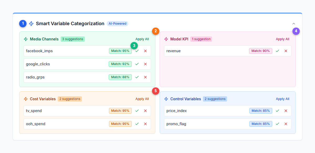
| # | Element | Description |
|---|---|---|
| 1 | Smart Variable Categorization header | AI-powered card with blue top border, appears automatically when suggestions are available |
| 2 | Media Channel suggestions | Suggested media variables with Apply All button to accept the entire category |
| 3 | Confidence badge | Match percentage (e.g., 95%) showing how confident the AI is. Accept (checkmark) or reject (X) each suggestion |
| 4 | Model KPI suggestion | Detected KPI variable (e.g., “revenue”) with confidence score |
| 5 | Cost Variable suggestions | Detected cost/spend variables matched by semantic analysis |
Halo and Trademark Channels
For multi-brand models, you can mark channels as halo or trademark channels during variable selection.
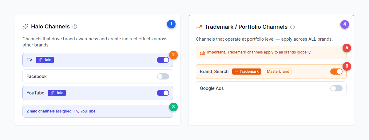
| # | Element | Description |
|---|---|---|
| 1 | Halo Channels panel | Mark channels that drive brand awareness and create indirect effects across brands. Indigo-themed with per-brand toggle switches |
| 2 | Halo badge and toggle | Active halo channels show a purple “Halo” badge. Toggle on/off per channel per brand |
| 3 | Halo summary | Shows count and list of assigned halo channels. At least one brand must have non-halo channels |
| 4 | Trademark / Portfolio Channels panel | Mark channels operating at portfolio level. Orange-themed |
| 5 | Global application notice | Trademark channels apply to ALL brands globally (not per-brand like halo) |
| 6 | Trademark badge and type | Active trademark channels show an orange “Trademark” badge plus a type indicator (Masterbrand, Portfolio, or Corporate) |
See Halo and Trademark Channels for detailed configuration guidance.
Step 4: Prior Builder
Configure prior distributions for each variable. The Prior Builder offers two modes.
Standard Configuration (Recommended)
The Standard tab automatically generates optimal priors based on your data patterns and industry benchmarks (FMCG, Retail, TelCo, Financial Services, E-Commerce). For a deep dive into how these defaults are calculated, see Smart Defaults.
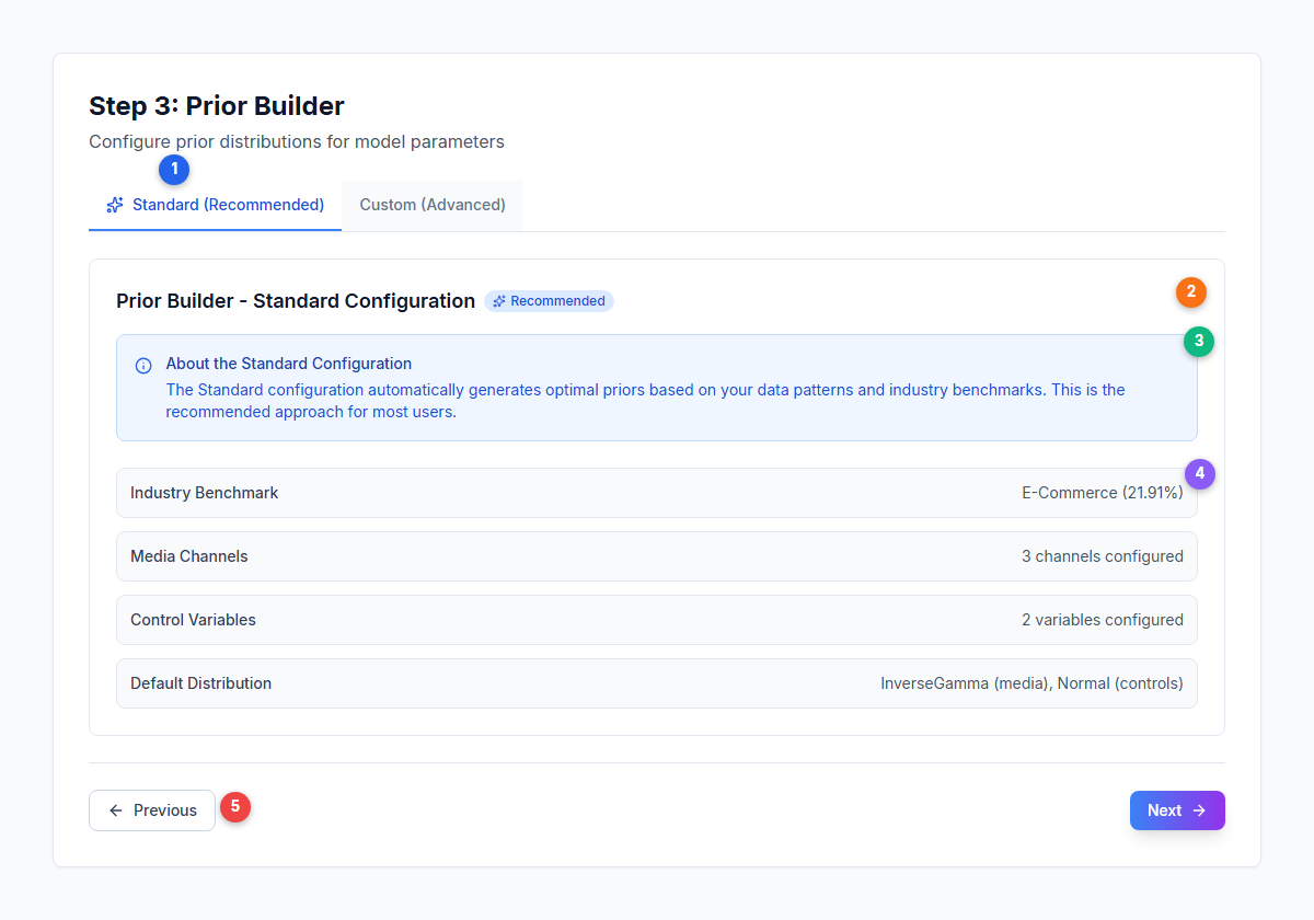
| # | Element | Description |
|---|---|---|
| 1 | Tab selector | “Standard (Recommended)” uses auto-generated priors. “Custom (Advanced)” enables manual editing |
| 2 | Configuration summary card | Shows the standard configuration with industry benchmark and channel counts |
| 3 | Info box | Explains that Standard mode automatically generates priors from data patterns |
| 4 | Summary items | Industry benchmark, media channel count, control variable count, and default distribution type |
| 5 | Navigation | Previous returns to Variable Selection, Next proceeds to Model Details |
Custom Configuration
The Custom tab exposes a full AG Grid table for manual prior editing. Each row represents a variable with editable parameters. For detailed guidance on choosing distributions, setting decay bounds, and tuning saturation parameters, see Model Configuration.
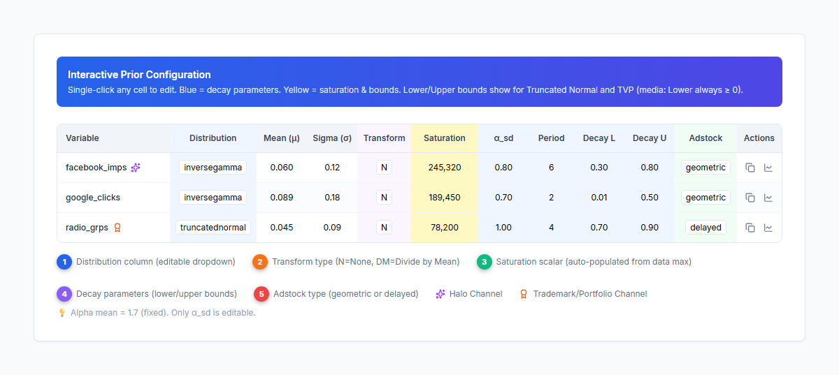
| # | Element | Description |
|---|---|---|
| 1 | Distribution column | Dropdown with four options: Normal, TruncatedNormal, InverseGamma, TVP (Time-Varying Parameter). InverseGamma is the default for media channels |
| 2 | Transform column | Data transform applied: N (None) for media, DM (Divide by Mean) for controls |
| 3 | Saturation column | Scalar value auto-populated from the maximum activity in your data. Controls the saturation curve scale |
| 4 | Decay parameters | Lower and upper bounds for the adstock decay rate (Beta distribution) |
| 5 | Adstock type | Geometric (immediate peak, exponential decay) or Delayed (peak after configurable lag) |
| ✦ | Halo Channel (purple sparkle icon) | Channels marked as halo get a fixed coefficient of 0.005 |
| ✦ | Trademark Channel (orange award icon) | Channels marked as trademark get 25% of their calculated prior |
Additional Custom mode features:
- Bulk Update: Copy settings from one variable to many using the Copy icon
- Graph Preview: Click the chart icon to see distribution shape and decay curves (uses Plotly.js for distributions)
- Master-Detail View: Alternative editing interface with keyboard navigation (J/K to navigate, Escape to close)
- Alpha mean is fixed at 1.7 (Gamma prior). Only alpha_sd is editable
Step 5: Model Details
Final configuration before fitting your model. This step brings together model naming, train/test splitting, advanced tuning options, and optional lift test calibration.
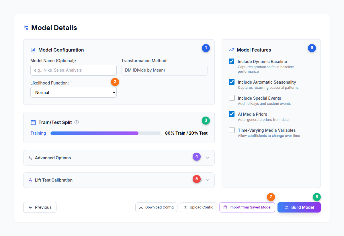
| # | Element | Description |
|---|---|---|
| 1 | Model Configuration | Set model name (optional), view transformation method (DM, fixed), and select likelihood function (Normal, LogNormal, StudentT, Quantile) |
| 2 | Likelihood Function | Dropdown controlling the statistical distribution for model fitting. Normal is the default |
| 3 | Train/Test Split | Slider from 50% to 100% training data. Default is 100% (no holdout test set) |
| 4 | Advanced Options | Collapsible accordion with seasonality, intercept priors, MCMC sampling, and diagnostics settings |
| 5 | Lift Test Calibration | Collapsible section for adding experimental calibration data (toggle to enable) |
| 6 | Model Features checkboxes | Right column (Custom mode only): Include Dynamic Baseline, Include Automatic Seasonality, Include Special Events, AI Media Priors, Time-Varying Media Variables |
| 7 | Config management buttons | Download Config, Upload Config, Import from Saved Model — save/load complete model configurations |
| 8 | Build Model | Submit the model for Bayesian inference. Enters the task queue |
Train/Test Split
Adjust what percentage of your data is used for training vs. holdout testing. A higher training percentage gives the model more data to learn from but leaves less for out-of-sample validation.
Advanced Options
The Advanced Options accordion contains four sections:
Seasonality:
- Annual Fourier terms: Default n=2 (range 1–25). Higher values capture more complex patterns
- Prior scale: Default 10, controls flexibility of the seasonality component
- Weekly seasonality: Only available for daily data, disabled by default, opt-in via checkbox (default n=3 terms)
Intercept Priors:
- Prior mean (default 2), lower bound (default 0), upper bound (default 2) — expressed as multiples of KPI mean
MCMC Sampling:
- Sampler: NUMBA (default, with progress tracking) or Nutpie (faster, no progress display)
- Target accept rate: Default 0.85 (range 0.6–0.99)
- Warmup iterations: Default 1,500
- Posterior samples: Default 1,000
Diagnostics:
- Sample from Prior: Generate prior predictive samples before fitting (useful for validating assumptions)
Lift Test Calibration
Add experimental results from geo-lift tests, conversion lift studies, or holdout tests to calibrate the model.
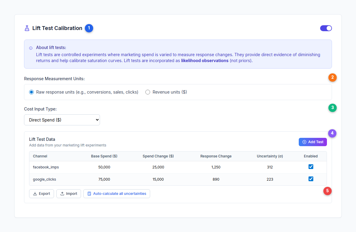
| # | Element | Description |
|---|---|---|
| 1 | Enable toggle | Turn lift test calibration on/off with the checkbox next to the section header |
| 2 | Response Measurement Units | Choose between raw response units (conversions, sales) or revenue units ($) |
| 3 | Cost Input Type | How to input test costs: Direct Spend, Cost per Acquisition (CPA), Cost per Click (CPC), Cost per Thousand Impressions (CPM), or Custom Cost Metric |
| 4 | Lift Test Data table | AG Grid for entering test data: channel, baseline level per period, change in level per period, response change per period, and uncertainty (sigma). Levels are in the channel’s own units, with the spend behind the change shown as context. Add new tests with the “Add Test” button |
| 5 | Add from a recorded test | Pick a test recorded under Warehouse → Experiments → Incrementality tests. Its row is derived for the model you are building and shown read-only under the grid; only the reference is stored. See Incrementality tests |
| 6 | Import/Export buttons | Export lift test data as JSON for reuse, or import a previously saved configuration. The “Auto-calculate all uncertainties” button is a placeholder that sets each row’s uncertainty to 25% of its response change; a recorded test’s interval is the better source |
Important: Lift tests are incorporated as likelihood observations (not priors). They provide direct experimental evidence that helps calibrate the model’s saturation curves and channel attribution. See Incrementality for the underlying methodology.
Holidays and Events
When “Include Special Events” is enabled in the Model Features checkboxes, a holiday selector appears:
- Country selector: Search 200+ countries, with popular shortcuts (US, GB, AU, CA, DE, FR, NL, IE, NZ, SG)
- Manual date picker: Add custom event dates
- Week convention: For weekly data, choose between “Week Commencing” (Monday) or “Week Ending” (Sunday)
- Holidays are automatically snapped to your data’s period boundaries and deduplicated
Import from Saved Model
The “Import from Saved Model” button opens a dialog to import posteriors and settings from a previously completed model:
- Variable Selections: Date, KPI, Media, Costs, Controls, Linked Items, Halo & Trademark Channels
- Priors: Posterior distributions converted to new priors (with adjusted scalars)
- Model Settings: Trend, Seasonality, TVP, Sampling options, Train/Test split
This is useful for warm-starting new models based on previous results.
After the Wizard
Once submitted, the model progresses through these statuses:
| Status | Description |
|---|---|
| Pending | Queued, waiting for compute resources |
| Under Way | Bayesian inference is actively running with a progress indicator |
| Complete | Results are available for review |
| Failed | An error occurred — common causes include insufficient data for the number of parameters, conflicting priors, or data quality issues. Check the error message and review your configuration |
| Revoked | Cancelled by the user before completion |
| Time Exceeded | Exceeded maximum computation time. Simplify by reducing channels, switching to weekly data, or disabling optional features (seasonality, trend) |
You can navigate away during fitting and return when it completes. Check status from the Warehouse or Dashboard.
Once your model completes, proceed to Incremental Measurement to interpret channel contributions, response curves, and model diagnostics. To optimize your budget based on the results, see Budget Optimization. For what-if forecasting, see Scenario Planning.
Next Steps
Platform guides:
- Model Configuration — Detailed prior and parameter tuning
- Smart Defaults — How auto-generated priors work
- Incremental Measurement — Interpreting your model results
- Budget Optimization — Optimize channel spend allocation
- Scenario Planning — What-if forecasting and scenario analysis
- VAR Models — VAR-specific model creation and analysis
- Halo and Trademark Channels — Cross-brand channel configuration
- Data Requirements — Data preparation guidance
Core concepts:
- Bayesian Modeling — Priors, posteriors, and the 94% HDI
- Priors and Distributions — Distribution choices and their implications
- Saturation Curves — Diminishing returns modeling
- Adstock Effects — Carryover and decay mechanics
- Seasonality — Fourier terms, trend, and holiday effects
- Halo Effects — Cross-channel and cross-brand spillover
- Incrementality — Lift test methodology and causal attribution